
How to compile WEEKLY Stripe Spreadsheet for the monthly Treasurer’s Report
Step One
Log in to Stripe Account. You will be on the “Balances” page (purple in left menu).
Step Two
Make sure you are looking at correct deposit. This one $215.66 on 01/02/2024.

Step Three
Scroll down until you see “Transactions”. On the right you will see “Export”. Click that block.

Step Four
When the Export is done, you will see this screen. It will give you the name of your export file (transfers(16).csv) that you will find in your downloads folder. Click “Close” in the export box.
Note that this is a .csv (comma separated value) file. You will convert to a .xlsx file in the next step.

Step Five
Open your Excel Spreadsheet Application. Click File>Open or touch “Command o” to get the next screen

Step Six
Click “Downloads” in the left gray menu and choose your transfer file to open it. You can either double click it or highlight it and click “Open” at bottom right of box.

Step Six-A
From now on, you will work in Excel. In the Excel menu, click File>Save As

Step Six-B
You will get a pop-up menu that has “Comma Separated Values (csv) highlighted. Scroll to the top of that box and highlight “Excel Workbook (.xlsx).

Step Six-C
In this box you will need to choose where you want to save the file and what name you want to give it. The assumption is you know something about Excel and file saving.
You will need to create a naming heirarchy for your Active Singles Treasury files. I suggest Documents>Active Singles Files.
If you are doing the weekly stripe report, I suggest you name it Stripe 010224 (where 010224 is the date of the Stripe deposit).

Step Seven
Your screen will look like this. Click the little half arrow in the cell just above cell 1 and to the left of cell A to highlight your full screen.
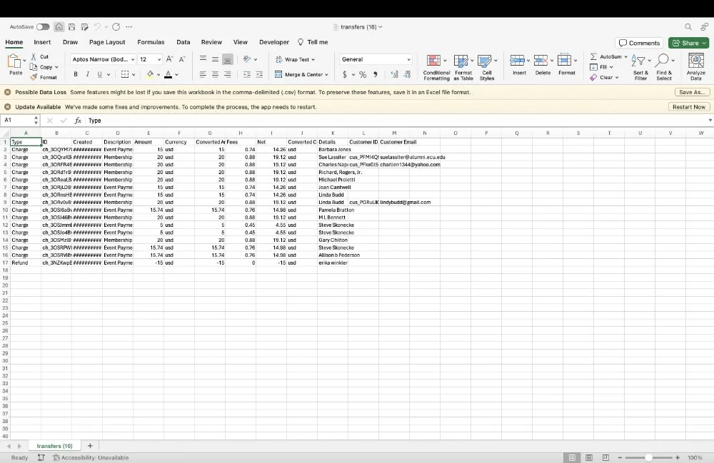
Step Eight
Make sure your whole screen is highlighted. On your “home” excel screen, click the little down arrow by “Format” (on the right) and click “AutoFit Column Width”

Step Nine
You can delete the following columns in Row 1: ID, Currency, Converted Amount, Converted Currency, Customer ID, Customer Email. Now format your Amount, Fees & Net columns to be currency with negative red.

Step Ten
Do formulas to get totals of columns: Amount, Fees & Net. Insure that the total of Net equals the deposit of the date you are working on.
